In this series of articles I’ll try to make a review of the current available analog modeling techniques that are used extensively both in hardware (digital stompboxes or pedalboards) and in software plugins.
I’ll do this by referencing a selection of academic papers on the argument and try to guess what kind of technology is used in current commercial products.
White-box vs black-box
-
White-box modeling is based on circuit analysis and simulation. Such models exhibit a high degree of accuracy, but require detailed knowledge of the circuit and its nonlinear components.
-
Black-box modeling is based on input-output measurements of the device under study. Black-box can be used to emulate different nonlinear systems, but it typically fails to emulate the system as accurately as a white-box model, leading to an audible difference between the model and the device under study.
The problem
Historically, the first approach that has been used and investigated by audio effects programmers was white-box modeling, because numeric methods to solve differential equations were already known for their application in circuit simulation programs such as Spice. The problem, with early implementations as well as today, is that processors don’t have enough computation power to solve the equations involved with such analog circuits (i.e. a guitar amplifier) in real time, or if you prefer complete the calculation of each voltage or current in the circuit nodes at the frequency requested by an high quality A/D to D/A conversion. That’s why various techniques to aproximate the solution of the most complex parts of the analog circuits have been developed. And that’s why we are always referring to the digital as a simulation, with people that claims for audible differences between analog circuits and their digital counterparts.
Waveshaping
In a paper from 1979 [1] this technique and its application in music synthesis was described for the first time. Since it’s simple in concept and very fast to compute, this method is still widely in use today. The audio source is passed through the transfer function in the figure below, which resembles what happens in real distortion circuits:

it’s common to refer to the family of these functions as ‘static nonlinearities’. Since you can have pretty much an infinite number of functions with a shape similar to this, and since you can combine them with extensive filtering in pre and post (or you can apply a different function for each frequency band), the problem relies in isolating the functions that sound good when applied to a guitar signal.
Physically-informed waveshaping
A non-linear analog circuit such a guitar amplifier (JTM45) or a stompbox (TS9) can be approximated by dividing it into blocks, separating the linear part, that can be represented by a n-order IIR digital filter from the nonlinear part which can be be obtained from numerical solution of the circuit [2]. For example see the figure below representing the TS9 overdrive effect:
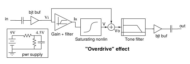
the distortion characteristic of the TS9 has been implemented with a static nonlinearity, this time derived directly from the equations of the circuit. Notice a portion of the ‘clean’ signal is mixed back with the distorted one: it’s typical of overdrive effects and is a major difference with distortion effects where the signal is not splitted and passes 100% through the nonlinear stage.
Approximation of a nonlinearity as ‘memoryless’ or ‘static’ is a straightforward technique, but has its limits.
In real analog circuits we usually have one or more reactive components (capacitors, inductors) being part of the differential equation that describes the nonlinear behaviour. Sometimes they are physical components, like in the next proposed example, but they could also be present in the form of parasitic capacitances/inductances.
For example, looking at the figure below, you can see that Vo is the voltage accross C and thus the output voltage depends on the ‘history’ of the input signal:
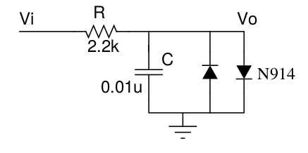
To model the nonlinear transfer function as static, the circuit is approximated by eliminating C. This simplification leads to a deviation from the original response of the real circuit, since we’re loosing the phase rotation introduced by the capacitor. A workaround for this specific circuit exists and will be discussed in a following article. In general terms, it’s important to measure such deviations during algorithm design.
If we keep deviations sufficiently low, that in audio terms means below the noise floor of the original circuit, then the digital version will be indistinguishable.
Aliasing
While discussing about waveshaping techniques in digital effects, we forgot to mention the elephant in the room, the aliasing problem.
Distortion adds or emphasizes harmonics in the original signal. But this also means that the base band of the original signal is expanded. If the new harmonic content introduced by the nonlinear function exceeds the Nyquist frequency of the system, the aliasing effect may become audible: without being too much technical, let’s say aliasing is when
one or more artifacts that sound unpleasant and unnatural are produced, unintentionally.
If you are interested in the sound of aliasing artifacts there’s a video here.
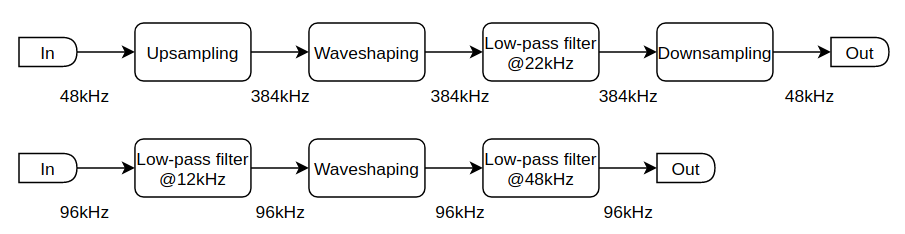
To avoid aliasing we need to introduce an upsample block before the nonlinear function and a downsample block immediately after. So if the system sampling frequency is 48kHz, internally the algorithm elevates it to 96kHz (2x) 192kHz (4x) or 384kHz (8x). The scope of the downsample block is the opposite: to return back to the original system sampling frequency (48kHz) for compability.
Upsampling is a CPU-intensive task, because the algorithm will run at 2x, 4x or 8x speed. Since the guitar’s voice is well below 12kHz (someone says 6kHz) we can avoid upsampling by introducing a low-pass filter before the nonlinearity. In addition to that we can rise the overall system sampling frequency to still have the 8x factor (96kHz/12kHz=8).
The following image summarizes the two approaches:
What’s next
In the next articles we’ll discuss, among others, about:
- Wave digital filters
- Profiling
- Deep learning
APPENDIX
A more detailed mathematical analysis is out of scope for this article, and will be the central topic in next articles, together with code examples, implementation ideas and so on. Please continue reading and supporting us thanks!
- C. Roads. A Tutorial on Non-linear Distortion or Waveshaping Synthesis.
- T. Yeh, J. Abel, and J. O. Smith. Simplified, physically-informed models of distortion and overdrive guitar effects pedals.